Context #
Note: An extended version of this has been accepted to the Mech Interp Workshop at ICML as well as the Workshop on Compositional Learning (how fitting!): Safety, Interpretability, and Agents at ICML. Look at it here: https://icml.cc/virtual/2026/69329.
This is a writeup of the part of our Algoverse Fellowship project that I worked on most directly: the circuit analysis and SAE experiments for a toy entity-binding transformer. The project was collaborative with Susie Park and Kushal Jain, and was mentored by Bart Bussmann and Patrick Leask (both MATS alumni). It was the first full mech interp project for the three of us, and a lot of what’s here owes to Bart and Patrick.
The motivation for this project came from Wattenberg & Viegas’ Relational Composition in Neural Networks: A Survey and Call to Action, which argues that feature-based interpretability is incomplete unless we also understand how models represent relationships between features. A model does not only need vectors for individual entities and attributes; it needs some way to represent which entities are bound to which attributes. For example, in a context like “Alice lives in Paris; Bob lives in London”, the model needs to keep track of lives_in(Alice, Paris) and lives_in(Bob, London), not just the unordered set of names and cities. This matters for SAE-style interpretability because compositional mechanisms can create feature multiplicity, echo features, or “dark matter”: relational information that is present in the model but hard to recover as a clean monosemantic feature.
A concrete version of this problem appears in entity-binding work. Feng & Steinhardt’s How do Language Models Bind Entities in Context? found evidence that language models use binding-ID-like vectors to connect entities with attributes in context, and Prakash et al.’s Fine-Tuning Enhances Existing Mechanisms: A Case Study on Entity Tracking later traced an entity-tracking circuit more mechanistically. But the question that interested us was slightly different: if a model uses a binding or address vector, how is that vector constructed in the first place?
In this project, we studied that question in a small synthetic transformer trained on entity-relation-attribute facts. The project had two goals: first, reverse-engineer the circuit the model uses for retrieval; second, train SAEs at relevant hook points to see whether they recover the relational structure or fail in instructive ways.
Task #
We trained a small 2L2H attention-only (d=256) transformer on 16M synthetic entity-binding samples until it reached 100% validation and test accuracy. Each prompt contained 5-8 facts of the form (E1 R E2 ,), followed by a query (R E1 ?). The model’s job was to return the matching E2. All results below are computed on a held-out test set of 8k prompts.
One small design choice mattered: we queried with (R, E1, ?) rather than simply repeating the fact order as (E1, R, ?). This was meant to avoid making the task too close to induction-head-style pattern matching. The model had to bind an entity and relation to the correct value, rather than just continue a repeated token pattern.
A staged retrieval circuit #
1. Probes localize the variables #
First, I used linear probes to ask where the task variables are represented after Layer 0.
The probe pattern was clean. At comma positions, L0H1 carries the value/content variable E2: E2 is not decodable
from blocks.0.hook_resid_pre (1.13%, essentially chance over 100 classes), is not decodable from L0H0, but is
decodable from L0H1 and blocks.0.hook_resid_post with 100% accuracy.
By contrast, L0H0 carries the address-side variables. E1, R, and the joint (E1, R) are all linearly decodable
from blocks.0.attn.hook_z, head 0, with 100% accuracy. On the query side, the queried entity and relation are also
decodable at the ? position from L0H0.
So Layer 0 appears to split the problem into two streams: an address stream (E1, R) and a content stream E2.
| Target | Position | Activation site | Accuracy |
|---|---|---|---|
| E2 | comma | blocks.0.hook_resid_pre | 1.13% |
| E2 | comma | blocks.0.attn.hook_z, head 0 | 0.0% |
| E2 | comma | blocks.0.attn.hook_z, head 1 | 100.0% |
| (E1, R) | comma | blocks.0.attn.hook_z, head 0 | 100.0% |
| query E1 | ? | blocks.0.attn.hook_z, head 0 | 100.0% |
| query R | ? | blocks.0.attn.hook_z, head 0 | 100.0% |
2. The address vector is additive #
The probe result says that L0H0 contains the address (E1, R), but it does not tell us how this address is
represented. It could be a lookup table with a separate vector for every entity-relation pair, or it could be composed
from separate entity and relation components.
To test this, I collected the L0H0 hook_z vector at every comma position and grouped activations by their (E1, R)
pair. For each of the 1,000 pairs, I computed the mean address vector and compared it to an additive prediction:
This explained 99.8% of the pair-level variance (FVE = 0.998). The mean cosine similarity between actual and predicted address vectors was 0.9996, with a minimum of 0.9921.
So the model did not learn an arbitrary address vector for each (E1, R) pair. The address is almost exactly a shared
mean plus an entity component plus a relation component.
3. Layer 1 retrieves the matching fact via QK attention #
After Layer 0 has written address representations at the comma positions and a query representation at the ? position,
Layer 1 has to select the fact whose address matches the query. In transformer-circuits terms, this is the role of the
QK circuit: it determines which source positions the attention heads read from.
I measured the query-key dot products between the ? token and all preceding comma tokens. Same-head matching was
highly reliable. For L1H0, the query at ? selected the correct comma key in 100% of test prompts, with a mean margin
of +103.2 over the strongest incorrect comma. L1H1 showed the same pattern: 100% top-1 retrieval, with a mean margin
of +102.5.
Cross-head pairings did not retrieve the correct fact, with top-1 rates near chance and negative margins. This suggests that retrieval is implemented by same-head QK matching between the query representation and the address representations at comma positions.
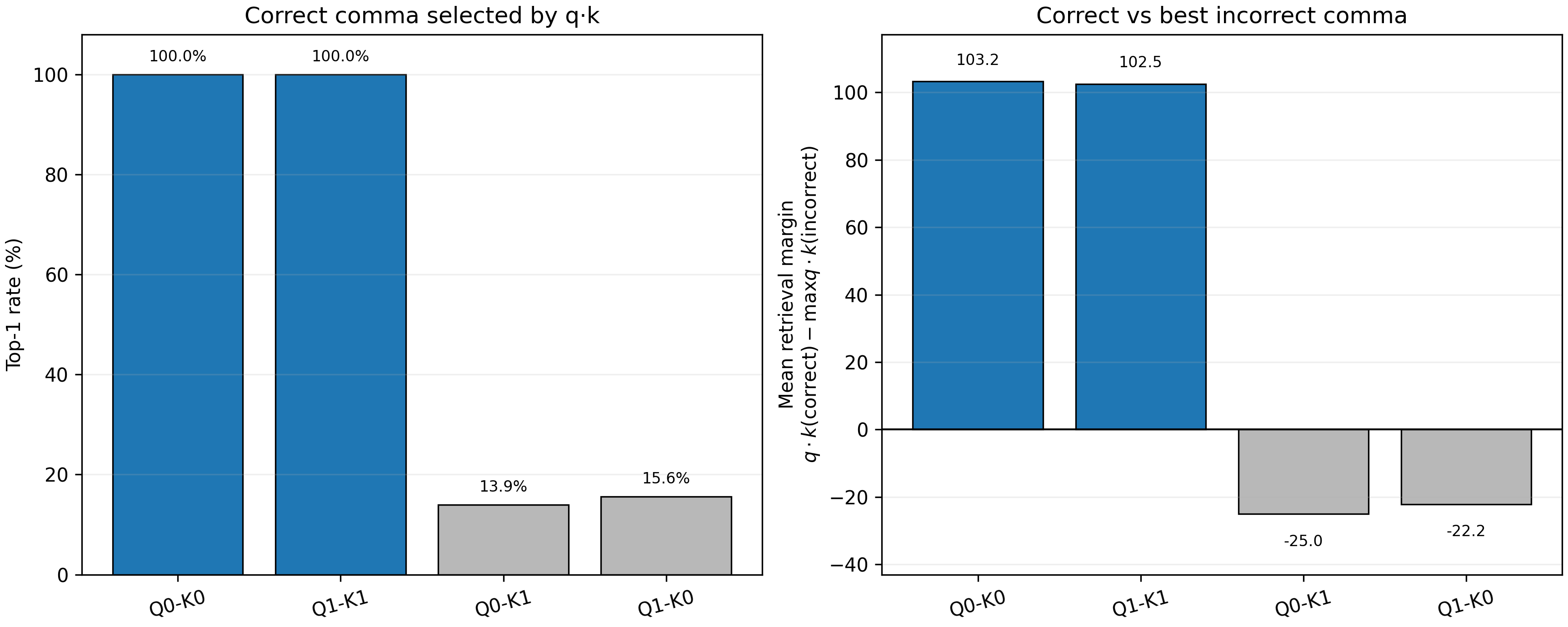
Layer 1 query-key matching. Same-head QK pairings select the correct comma in 100% of test prompts and produce large positive retrieval margins, while cross-head pairings fail to separate the correct fact from distractors.
4. Causal interventions confirm the address/content split #
The probe and QK analyses are correlational, so I also tested whether the address representation causally controls which value gets retrieved.
# 1. Address relocation only
logits_relocate = model.run_with_hooks(
    tokens,
    fwd_hooks=[
        ("blocks.0.attn.hook_z", replace_distractor_address),
    ],
)

# 2. Address relocation + original target corruption
logits_relocate_and_corrupt = model.run_with_hooks(
    tokens,
    fwd_hooks=[
        ("blocks.0.attn.hook_z", replace_distractor_address),
        ("blocks.0.attn.hook_z", corrupt_target_address),
    ],
)
The intervention was to move a target-style L0H0 address vector onto a distractor comma. On its own, this made the
model uncertain between the original target and the distractor. But when I also corrupted the original target address,
the prediction flipped decisively to the distractor. The mean logit difference moved from strongly favoring the original
target (-24.46) to strongly favoring the distractor (+24.49).
This supports the address/content interpretation: changing the address changes which slot Layer 1 retrieves from.
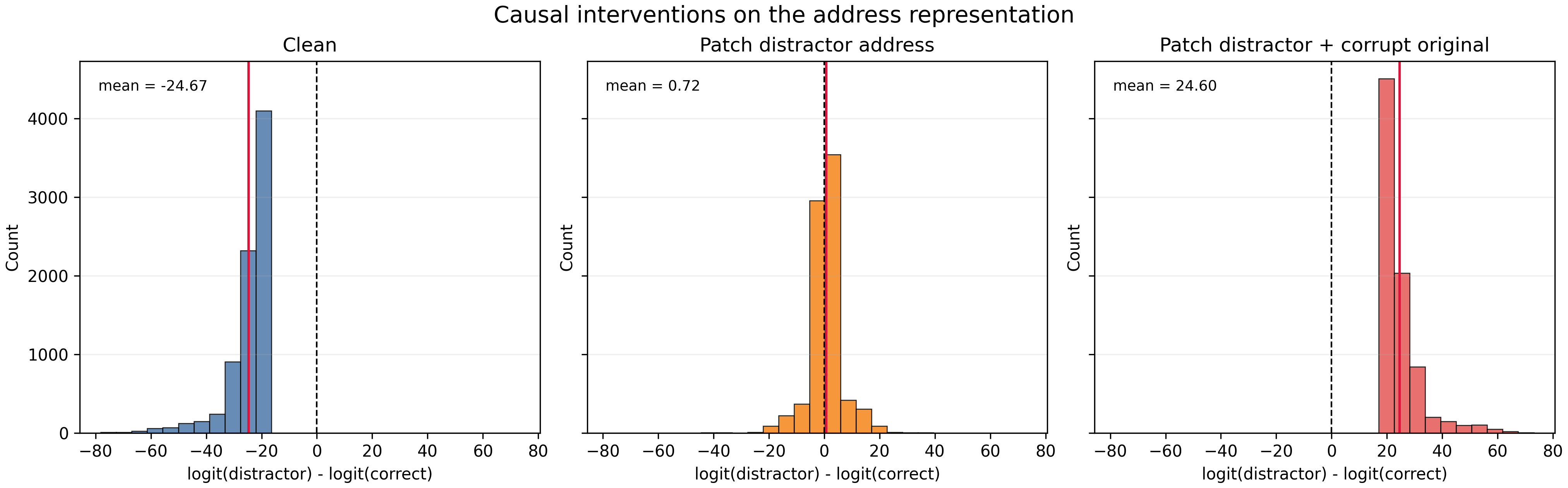
Causal interventions on the address representation. Relocating the target-compatible address to a distractor comma makes the model uncertain; relocating it while corrupting the original target address flips the prediction to the distractor.
5. Putting it together #
Putting these pieces together, the model implements a staged retrieval circuit. Layer 0 writes an additive address representation (E1, R) and a content representation E2 at comma positions. Layer 1 uses a same-head QK circuit to select the comma whose address matches the query, after which the corresponding content is propagated to the output.
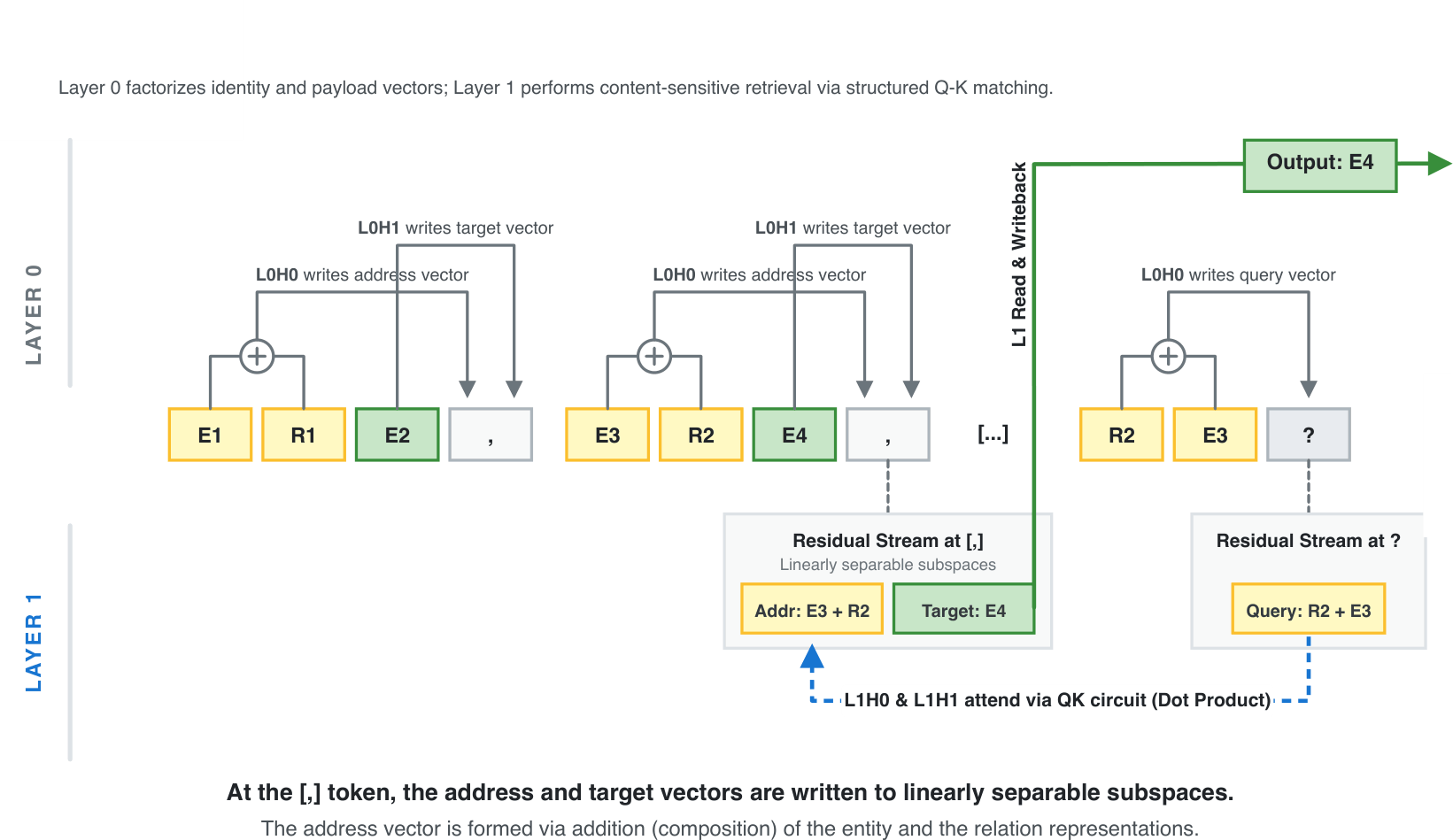
Full staged retrieval circuit. Layer 0 writes address and content representations at comma positions, then Layer 1 matches the query against the address and retrieves the corresponding content.
SAE feature recovery #
We also trained SAEs to test how well SAE-style feature discovery would recover the variables used by the circuit.
We trained BatchTopK SAEs with 1024 latents and k=8 at two comma-position activation sites: blocks.0.attn.hook_z, head 0, where the address representation is still isolated, and blocks.0.hook_resid_post, where the Layer 0 outputs have been combined into the residual stream. We analyzed the 1M-step checkpoints. Both had high reconstruction quality: fraction of variance explained (FVE) was about 0.999 for L0H0 hook_z and 0.997 for resid_post.
To evaluate feature recovery, we used best-F1. For each target class, we selected the SAE feature that best identified that class, then averaged the resulting F1 scores across classes.
At the L0H0 hook_z address site, the SAE partially recovered the factorized address-side variables. E1 reached mean best-F1 = 0.585 and R reached mean best-F1 = 0.778. However, this did not amount to one clean latent per full address (E1, R), and recovery was far weaker than the 100% linear-probe result.
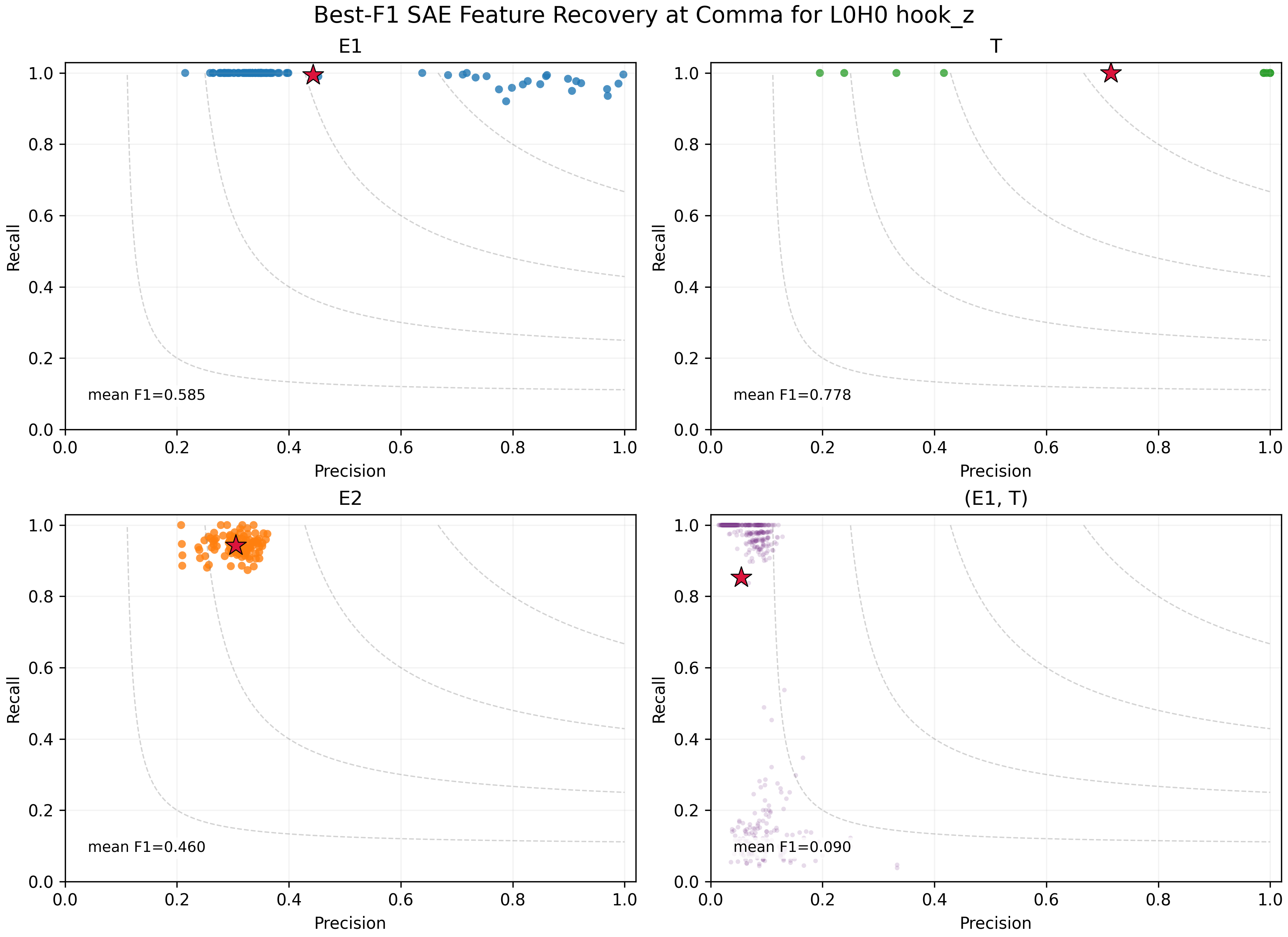
SAE feature recovery at the L0H0 address-head output. Entity and relation factors are recoverable, but not as one clean latent per full address.
At the combined resid_post site, the SAE recovered the payload variable E2 very cleanly, with mean best-F1 = 0.958. Address recovery was much weaker. Although a direct linear probe gets 100% accuracy on the joint (E1, R) address from the same activation site, the mean joint-address best-F1 was only 0.195.
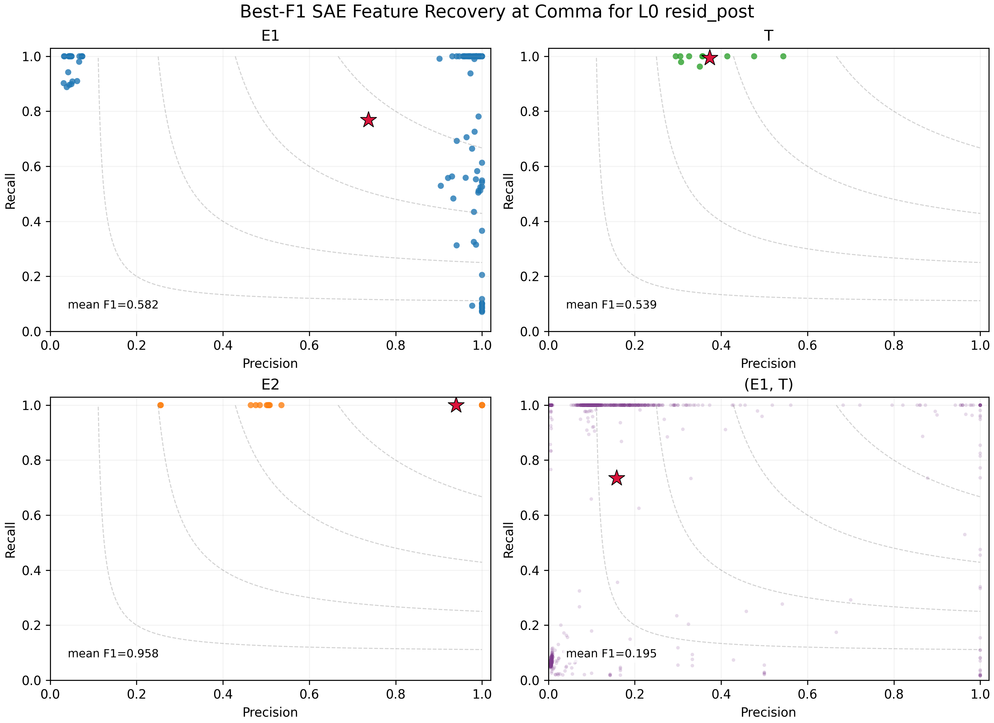
SAE feature recovery after Layer 0 composition in the residual stream. Payload recovery is clean, while address-side recovery becomes much less compact.
The main result is therefore less clear: The SAEs found some pieces of the structure, but did not give the same clean mechanistic picture as probes, patching and QK analysis. This points in the direction of the dark-matter concern from Wattenberg & Viegas: relational information can be present, linearly decodable and causally important while still not appearing as a small set of clean sparse features at the activation site being analyzed.
Discussion #
We show that our toy transformer learned a clean staged retrieval circuit for entity binding. Layer 0 separates the problem into an address stream and a content stream: L0H0 writes an address representation for (E1 R), while L0H1 writes the corresponding payload E2. Layer 1 then uses same-head QK matching to select the comma whose address matches the query. Here, the address is constructed almost exactly additive, by adding the E1 and R representations to a shared bias term.
The SAE results were less clean, but still useful. The address information was linearly decodable and causally important, yet it did not consistently appear as a small set of clean sparse features, especially after the Layer 0 outputs were combined in the residual stream. This is not a full dark-matter result, but it is a small example of the concern: relational structure can be present in the model while being harder to recover with standard feature discovery than with probes, patching, and circuit analysis.
The main limitation of this work is that we focused on a toy model. The natural next step would be to extend this to larger language models and see if similar behavior can be observed there.